
Should All Depressed Patients Be On Adjunctive Mirtazapine?
Explaining heterogeneity, tau, and random-effects models to better understand the meaning of a meta-analysis on combination therapy

Over the past couple of decades, a lot of the common psychiatric dogmas around antidepressant prescribing for depression have not held up well.
Shouldn’t we push the dose as high as can be tolerated before declaring treatment failure?
Probably not.
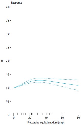
Furukawa et al. (2019) showed that for most commonly used SRIs1 and mirtazapine, dose equivalents beyond 20-40mg of fluoxetine do not show better efficacy. Only venlafaxine showed increasing efficacy with dose increases to the upper end of its dosing range. In other words, we should be sticking to the low-to-moderate end of the dosing range.
For patients who don’t respond to low-to-moderate doses, it’s at least worth a try to push the doses higher, right?
Doesn’t look like it.
Dold et al. (2017) found that increasing antidepressant dose did not improve HAM-D scores in patients with unipolar depression across 7 RCTs. There was no effect of baseline symptom severity on effect sizes in their meta-regressions:
Dose escalation was not more efficacious in HAM-D total score reduction than maintaining standard-dose treatment, neither for the pooled antidepressant group (N = 7, n = 999; Hedges g = –0.04, 95% CI: –0.20 to 0.12; p = 0.63 [I2 = 10.4%]) nor the individual antidepressants.
Didn’t STAR*D show that we can switch to another antidepressant or augment and people should get better?
STAR*D has… a lot of methodological problems. The critique and re-analysis by Pigott et al. (2023) points out that the authors did things like:
Excluding from analysis, 370 patients who dropped out after starting on citalopram in their first clinic visit without taking the exit HRSD despite STAR*D investigators stating, ‘our primary analyses classified patients with missing exit HRSD scores as nonremitters a priori’
Including in their analyses, 125 patients who scored as remitted at entry into their next-level treatment. This occurred despite STAR*D investigators prespecifying that ‘patients who begin a level with HRSD<8 will be excluded from analyses’
After re-analysis, the Pigott authors found that real remission rates in STAR*D were probably between 35-41%, much lower than the 67% STAR*D’s authors claimed, which has now become “common knowledge” in psychiatry. For this, and many other reasons, we can’t really rely on STAR*D for good guidance about effective prescribing practices.
Ok, So What About Switching?
Bschor et al. (2018) finds no benefit:
…switching was not superior to continuation: the standardized mean difference in the strict analysis was −0.17 (95% CI, −0.59 to 0.26; P = .45; I2 = 77.8%) and in the broad analysis was 0.031 (95% CI, −0.26 to 0.32; P = .836; I2 = 85.3%)
Though, to be honest, the data here is quite sparse, and those I2 statistics should give you pause, particularly after you read this essay. This is the weakest of the null findings in my view.
Dare I Even Ask About Augmentation?
Fortunately, current evidence suggests that augmentation might actually do something! There are meta-analyses suggesting benefit for augmentation with lithium, aripiprazole, and a few others.
Today we’re going to focus on adjunctive treatment with α2 antagonists2 using a relatively recent meta-analysis.
Henssler et al.
Combining Antidepressants vs Antidepressant Monotherapy for Treatment of Patients With Acute Depression: A Systematic Review and Meta-analysis is a 2022 meta-analysis by Henssler et al., published in JAMA Psychiatry which served as an update to a 2016 meta-analysis regarding the effectiveness of antidepressant monotherapy vs. combination therapy in patients with major depressive disorder.
In their survey of the literature, the authors looked for RCTs that met the following criteria:
Intervention using a combination of two antidepressants (i.e. no antipsychotics) regardless of dosage.
A control group of patients on antidepressant monotherapy
Ages 18 years and up
Depressive disorder “diagnosed according to standard operationalized criteria.”
Studies were excluded if they:
Solely focused on bipolar depression
Were purely maintenance trials
Clearly the authors are trying to cast a wide net here, which is understandable, but if we’re going to be thinking about heterogeneity we need to understand the sorts of studies that were allowed. Here are a couple of examples that the authors themselves point out in their methods:
There was no exclusion for other comorbid psychiatric or medical disorders
Trials could be of “first-line” treatment or in patients who had failed monotherapy.
All told, they came up with 39 studies that met their inclusion criteria.
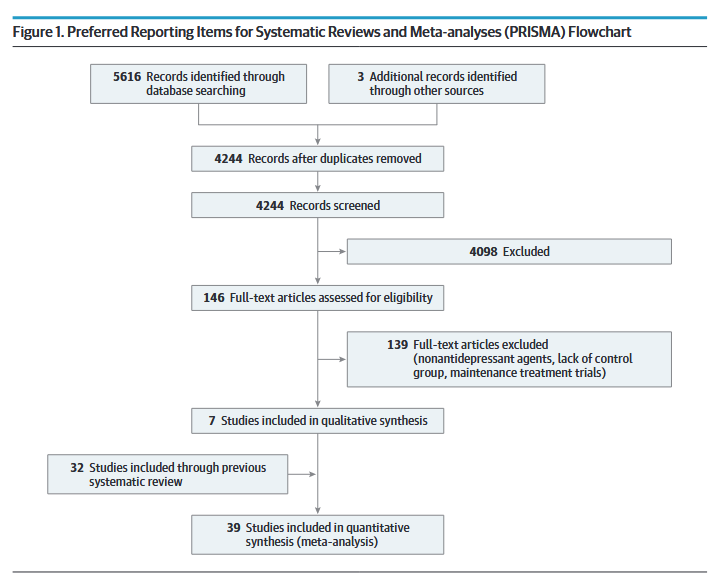
These studies spanned from 1977 to 2020 and included a total of 6751 patients. 23 studies (59%) were double-blinded, 5 were single-blinded, and 11 were open-label.
Outcomes
On their primary outcome — treatment efficacy measured as the standardized mean difference (SMD) between combination and monotherapy — Henssler et al. find a SMD of 0.31 (95% CI 0.19 to 0.44, P < 0.001) in favor of combination therapy. This result is actually pretty uninteresting due to the subgroup analyses, which happen to have some very interesting results.
At least in my clinical milieu, much has been made about the analyses regarding the addition of either an α2-antagonist or bupropion, which I’ve isolated in a modified version of Table 2:
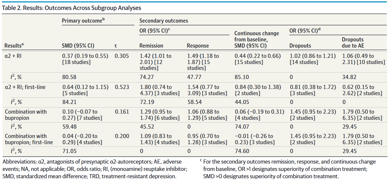
The message here is clear, right? Combination therapy with α2-antagonists is moderately superior to monotherapy, while bupropion augmentation doesn’t seem to do anything at all. Not only that, but — if you look at the rightmost two columns — combination therapy was tolerated just as well as monotherapy.
Looking at another adaptation of Table 2:
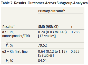
We might conclude that α2-antagonist combo therapy is superior to monotherapy as a first-line treatment and in nonresponders, though (unsurprisingly) less so in the latter group.
So, if we’re looking to maximize clinical response, maybe we should be starting all of our depressed patients on a SRI/SNRI + mirtazapine. Before you argue that you might want to start with monotherapy from a tolerability perspective, remember that there was no difference in dropout rates for adverse events between monotherapy and combination!
But… aren’t those I2 numbers pretty high? What is τ (tau) and what does it tell us? Do these numbers change anything about how we should interpret the results?
So glad you asked.
Running An Antibiotic Trial
Before we get there, to really understand what I2 means, I need to lay a little statistical groundwork.
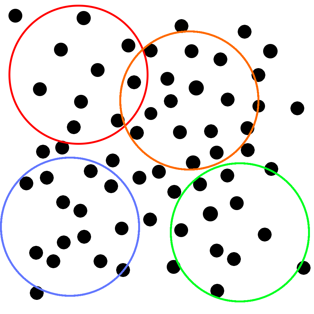
Imagine that you’re trying to study how quickly a new antibiotic resolves upper respiratory symptoms. You’ve collected your study subjects, lured invited them into a room, assigned them to specific positions, and told them that they won’t get their honorarium if they leave.3 Here’s a representation of where they are in the room:

Unfortunately, due to budgetary constraints, each individual study can only include the number of people that you can encircle with an unusually large hula-hoop. That you throw with your eyes closed. You know, so your throws fall completely randomly.
Corporate has generously decided to give you enough money to throw the hoop four whole times. Yay! Your perfectly random throws fall like this:
With each of these samples, you do four very high quality RCTs that are all roughly identical from methodological standpoint. You make some tweaks around the edges, but you’re not worried too much. You know that all upper respiratory symptoms are caused by bacteria (you’ve seen those ads on the subway) and how many types of those can there be? Two? Three?
Unfortunately, the editors of the last journal you sent your manuscript to said that just averaging the numbers from your studies and writing “THIS IS A META-ANALYSIS” in your methods section wasn’t good enough. So, you used the money you saved from not paying the participants you missed with the hula hoop to hire a statistician.
The statistician, after looking through your previously submitted manuscripts with a concerned look on her face, explains that your statistics need to account for this thing called heterogeneity. She tells you that this is because, even though your antibiotics are very strong and there are probably only three types of bacteria (is there a hint of condescension in her tone?) we need to be confident that the differences in the results between studies are due to sampling error and not because your studies are measuring different “true” effects.
Why Did You Put “True” In Quotes?
Let’s assume, the statistician says, that the people you put into the room were the only people in the world with upper-respiratory symptoms; we can call them a population that you might take samples from. We take as true that their symptoms are caused by bacteria and that the antibiotic treats them equally as effectively. Finally, also assume that you did all of your studies equally well and there are no major differences between them that would have a significant impact on the results.
Now, imagine that corporate gave you a hula-hoop that was big enough to encircle everyone in the room at the same time,4 so that you could just do one big study on the entire population (i.e. your sample = your population). The mean (μ) and distribution (described by a standard deviation (σ)) of symptom improvement from that study would be what we might call the “true” effect of the antibiotic in the population of individuals with upper-respiratory symptoms caused by bacterial infections.
As a brief aside here. I think it’s important to address that a “true” effect of an intervention is a partial fiction that depends on how you define your population. When we talk about how an antihypertensive that lowers blood pressure, there is a single “true” effect size in the population of adults with hypertension, but there is also a separate “true” effect size of this medication in adults >65 with hypertension. And another for female adults >65 with hypertension. And another for African American female adults >65 with hypertension living in the state of North Carolina. And another for all Americans regardless of whether or not they have hypertension. See what I’m getting at here?
Of course, you only had the one smaller hoop that corporate gave you, so you only have four randomly selected samples of the room’s population. If we graph the probability distributions of the first two samples (Study 1 and Study 2) alongside the distribution for the whole room we might see something like this:
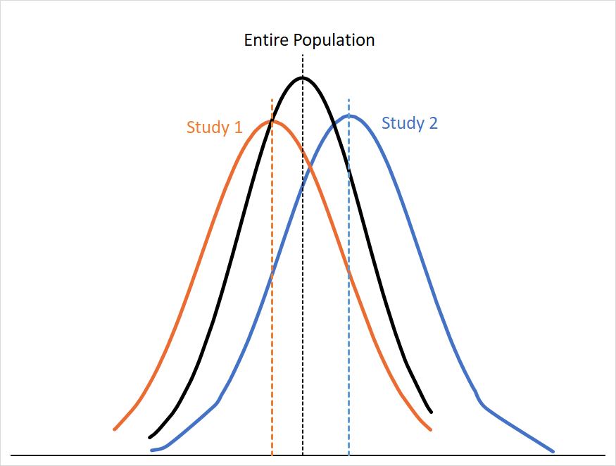
You can see that the curves for Study 1 and Study 2 approximate the curve for the entire population, but not entirely. If our assumptions about the population in the room still hold (e.g. no meaningful differences in efficacy, study design, etc. ) we can assume that these differences are because of sampling error. Sampling error arises from the fact that any sample is only a subset of that population, so your result is almost always going to skew a little high or low relative to the “true” mean.
Sampling error gets smaller the more people you have in your sample size; this makes sense, since you’re just getting closer and closer to sampling everyone in the population. You can see this if we were to combine the data for Study 1 and Study 2:5
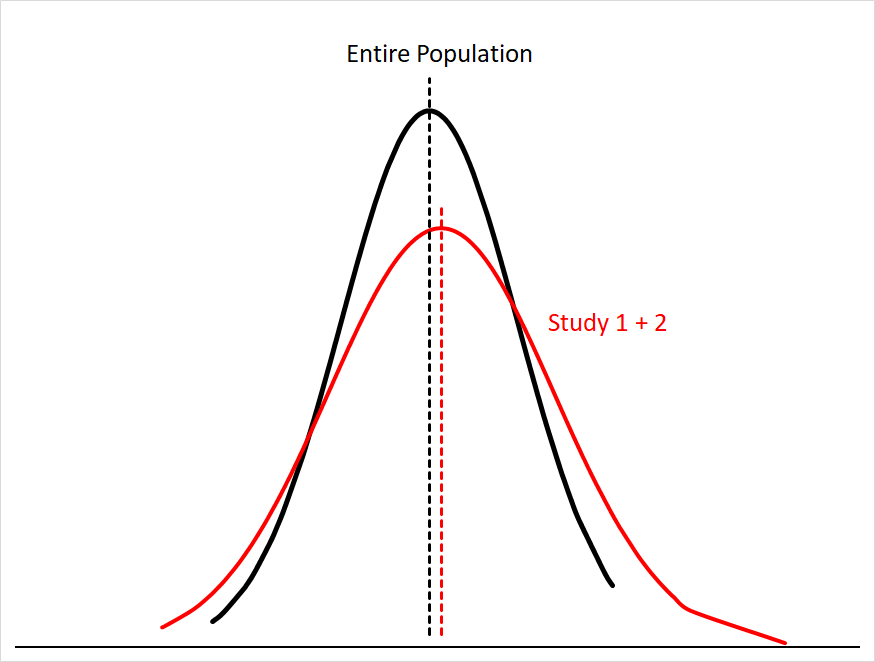
Our mean for the combined studies is now much closer to the population mean, and the area under both curves matches much more closely.
The problem, the statistician says, is that we can’t be confident in the assumptions we mentioned earlier. She leans in conspiratorially6 and whispers to you that she has learned about a cabal of doctors that say they are specialists in infectious diseases and claim that some upper respiratory symptoms are caused by things called “viruses” that aren’t even susceptible to antibiotics!
Imagine, she says, holding up a new picture, that the pink circles represent people who are actually infected with these “viruses”:
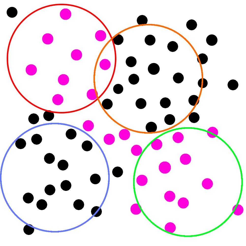
That’d be pretty bad! If this picture is real, two of your studies would be filled with people whose symptoms wouldn’t respond to antibiotic treatment at all.
In statistical terms, the population of people with viral infections would have a “true” response to the antibiotic totally different from those with bacterial infections. If you combined the data from those studies together in a meta-analysis, it might look something like this:
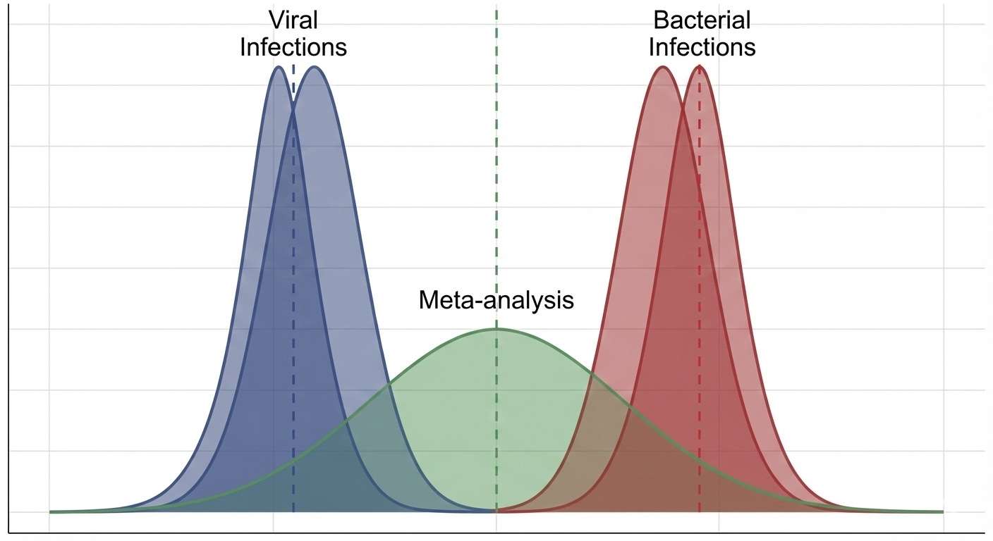
You can see why the statistician brought this up. Those “viruses” (if they exist) could make your antibiotic look much worse than it really is. Even worse, corporate might only let you throw the hula-hoop twice next time, and that was your favorite part of the whole thing!
Thing is, you already let all of those people go (the lawyers were pretty firm about this when they found out) and you didn’t even think to test them for viruses beforehand. In fact, now you’re starting to realize all of the other things that might make a difference. Maybe some of these people were at different stages of their illness. Maybe there’s a difference in how well this drug works depending on age. Maybe it matters that you started to run out of antibiotic after the first two studies, so you only gave half doses in the last two.
You could have dozens of different “true” effect sizes. Or just two. How are you supposed to know?
This is where heterogeneity (I2) comes in handy
To calculate I2 we use Cochran’s Q statistic, which measures how much the individual study estimates vary from the overall pooled estimate. You can think of Q as asking “Are these studies too different for the cause of that difference to just be sampling error?”
If there is no heterogeneity between our studies, we expect Q to equal degrees of freedom (df = # studies - 1). The bigger Q is relative to df, the more unexplained variance there is between studies. It is important to note that Q is very sensitive to precision. The more precise your studies are, the easier it is for Q to get very big.
With Q and degrees of freedom (df) we can compute I2 rather simply:
We can see that the numerator is just what remains after we subtract out the expected amount of sampling error (essentially df) contained in Q. If you look at the equation, you can see that this should be 0 if Q = df, which would give us I2 = 0%, which makes perfect sense since Q = df when there is only sampling error driving between-study differences.
We can see that the closer Q is to df, the smaller I2 will be.
In statistical terms, we can understand I2 as the proportion of total observed variability in effect estimates that is due to real between-study heterogeneity rather than sampling error.
Interpreting I2
A small I2 (0-25%) should suggest to you that the pooled effect size from your meta-analysis approximates one “true” effect size. That is, most of the differences you saw in the results were due to sampling error.
A large I2 (>50%) indicates that your pooled effect size is not representing a single “true” effect size, but a combination of different “true” effects that reflect meaningful differences in the characteristics of the studies included in the meta-analysis.
However, we can’t just use a large I2 to write off a meta-analysis as useless because I2 does not tell us anything about the magnitude of the range of “true” effects contained in our data. The differences in SMDs could be relatively small (e.g. +/-0.07) or very large (e.g. +/-0.7)
To illustrate this point, imagine that corporate let you run studies on millions of people — so your results are very precise (i.e. your confidence intervals are very narrow) — but your studies are limited to people either from Boston or LA.
Unbeknownst to you, people in Boston only get infected with Bacteria A, while people in LA only get infected with Bacteria B. The antibiotic works great on both, but they work slightly better on Bacteria A: The average person in the treatment group with Bacteria A gets better in 24 hours +/- 10 minutes while the average person with Bacteria B gets better in 26 hours +/- 10 minutes. Patients given placebo take an average of 14 days to recover.
After looking at the results, you’re confused. Your average effect is large and error is small (i.e. your study is quite precise). The antibiotic clearly works really well for both groups, but I2 is still very large! What gives?
This is because your large studies are (1) very precise and (2) are approximating two different “true” effects. This means that Q is very large, which means that I2 is very large. Imagine that you did 8 studies, and Cochrane’s Q = 100:
You’re still a bit confused, though. In this case it seems pretty likely that 93% doesn’t represent something clinically important — nobody will really care if there are two “real” effect sizes that differ by 2 hours — but what do we do in other studies with less precision? How do we express the magnitude of the heterogeneity relative to the SMD?
That’s why we have Tau (τ).
τau
As you might have guessed, τ is a way to express where the “true” effects of the various studies in your meta-analysis lie. It represents a standard deviation of “true” effects relative to the pooled SMD of your meta-analysis.
Normally, we’d just say that the 95% CI for “true” effects would be SMD ±2τ,7 but remember that we are pretty sure that the SMD in a highly heterogeneous meta-analysis represents some average of different “true” effects, so we need to be a little fancy and report a random-effects prediction interval (PI). The “random-effects” part means that we assume that every study represents a single “true” effect size, not a single fixed effect (more on this soon!). In English, a 95% prediction interval tells us the following:
If we did an additional study that was similar8 to the ones already included, then under this model, 95% of the time the new study’s “true” effects would lie somewhere in this prediction interval
Suppose that you have a meta-analysis of 10 studies that produces a SMD of 0.50 (95% CI: 0.25-0.75) and τ = 0.3.
If we just did the simple ±2τ method, we’d get a 95% confidence interval of (-0.1 to 1.1)
If we construct a prediction interval (I used this calculator) we get a 95% PI of (-0.223 to 1.223). This means:
If we did an additional study that was similar to the 10 already included in this meta-analysis, there is a 95% chance that the “true” effect of that new study will fall between -0.223 to 1.223.
You’ll notice that the PI is wider than the the simple ±2τ method, which makes perfect sense since the PI is also includes uncertainty about the SMD due to heterogeneity.
In the ultra-precise LA/Boston antibiotics study, you can see how τ and a PI would make you unconcerned about heterogeneity. Even if I2 = 93%, a small τ and a narrow 95% PI that indicates that 95% of your “true” effect sizes are within 2 hours of your SMD means that the heterogeneity in this study is clinically irrelevant.
Weighting Studies
Now that we understand some things about measuring and modeling heterogeneity in a meta-analysis, we can use this to better understand the two major models used to combine study outcomes in meta-analyses and their consequences for the results.
This is the last thing we need to understand before we get back to Henssler.
Intuitively, we know that some studies are “better” than others. Concretely, we might say that “better” studies are ones with a low risk of bias, higher precision, and so on. Regardless of how we define “better” we have decide how strongly to value one study relative to one another. i.e. we have to assign them weights.
Fixed Effects Modeling
If we want to conceptualize a single “true” effect size that all of these studies are pointing towards (let’s call this a fixed effect); studies with smaller variances give us more precise information about where that “true” effect size is likely to be. Consider how much more useful Study 1 is than Study 2 in narrowing down where the “true” effect is:
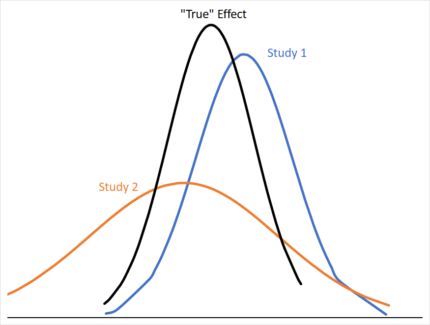
The mean effect of both studies are the same distance from the “true” mean, but Study 2’s 95% CI covers a far larger range of numbers with similar probabilities, and so is less informative about where the “true” mean is likely to be. Statistically, we can describe Study 2 as having a larger standard error (SE), which is calculated from its standard deviation (σ) and sample size (n) as follows:
SE estimates how much your sample mean would bounce around if you repeated the study many times.9
In cases where we want to think about individual studies as representing a population subject to a single “true” effect-size, we use a fixed-effects model to weight our studies. In a fixed-effects model, a study’s weight is expressed as:
In other words, studies with high variance/large SEs get weighted less and studies with low variance/small SEs get weighted more. Since a fixed-effect model assumes that there exists a single “true” effect, it would make sense that we would want to weight our more precise studies very highly, since they tell us the most about the location of the “true” effect size.
What if we don’t think that our studies are likely to represent a single “true” effect, because we’re studying a syndrome with poor construct validity, lots of possible etiologies, and the potential for wide ranges of responses to treatment depending on those etiologies?10
Random Effects Modeling
In that case we might use a random-effects model, where we assume that each study represents its own “true” effect size. i.e. we don’t assume that the differences between studies are just because of sampling error, but because of real differences between studies.
The equation for a study’s weight in a random-effects model is very similar to the fixed-effect equation: it’s the inverse of the variance plus τ2
Basically, τ2 sets a ceiling on how heavily large, precise studies get weighted, because SEs << τ2 turn into a rounding-error in the denominator. No study weight can ever be smaller than τ2.
Relative to a fixed-effects model, a random-effects model tends to decrease the weighting of large, low-variance studies, and increases the relative weight of small, high variance studies. Again, this makes sense if we don’t think that there is a single “true” effect; we wouldn’t want our large studies to totally dominate our SMD if we think that their effect is just one of many “true” effects.
It’s instructive to see an example to see just how big the swing can be, so why don’t we use the largest (Kato et al., n=1647) and smallest (Maes et al. (1996) n=22) studies from Henssler et al., so we can see how they look under fixed and random-effects models:
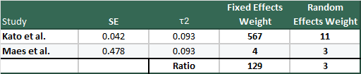
Hopefully this drives home how massive the difference between the weighting in the two models are, and why you might get concerned about small, high variance studies in meta-analyses.
Before we get off the differences between the two models, it is important to note that, in a random-effects model, the SMD of the meta-analysis takes on a different meaning. Instead of the SMD and 95% CI approximating a single true effect, the SMD in a random-effects model represents the average “true” effect of “true” effects in the included studies and a range in which those “true” effects fall.
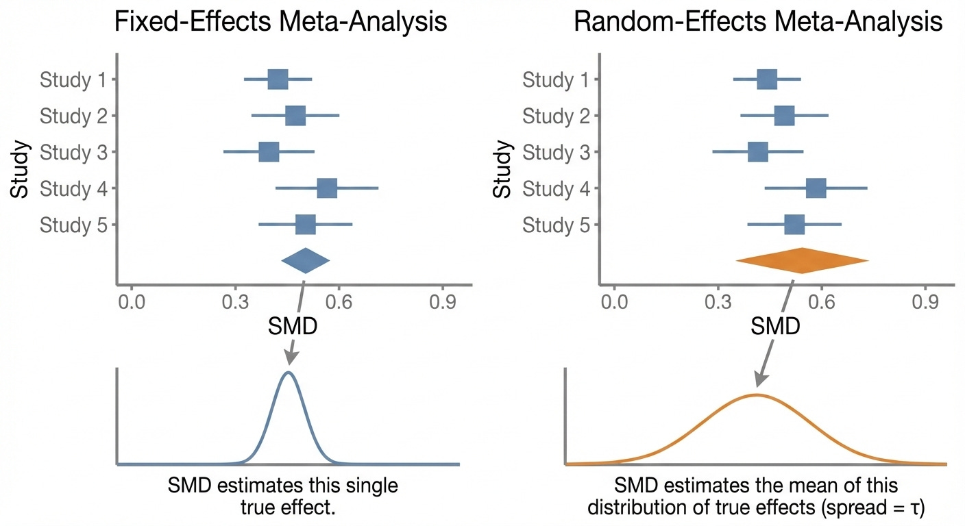
Neither of these models is necessarily “better” than the other, they just tell us different types of information. For example, even when dealing with a population that you know is very heterogeneous (e.g. MDD), a fixed-effects model might be more useful than a random-effects model from a clinical perspective if you don’t have any way to identify which patients fall into subpopulations likely to experience larger “true” effects.
They are also not the only models: there are quality-effects models (where studies are weighted by study-quality or risk-of-bias scores), Bayesian random-effects models, and more.
A Brief Recap
We’ve learned that to study an intervention, we take samples from a population of interest, perform an intervention, and measure the effects.
When we combine the data from these different studies in a meta-analysis, we take as given that there will be statistical differences in the results. What we need to understand is whether the differences in variance (SE) between our studies appear to be driven by sampling error or real differences between the studies.
Using Cochran’s Q, a measure of between-study variance that is very sensitive to precision, we can calculate I2.
I2 tells us what percentage of the variance in effect estimates is attributable to true between-study differences, but it does not tell us the size, spread, or directionality of those differences.
If I2 is small (<25%), it’s reasonable to assume that our included studies are constructed such that they are sampling from the same population and that they measured similar outcomes. In other words, we can be fairly confident that they are all approximating a single “true” effect size.
If I2 is large (>50%), we need to investigate whether or not the effects of heterogeneity on our meta-analysis is meaningful. We do this by (1) assuming that every study in our pooled analysis reflects its own “true” effect, and (2) calculating tau (τ) which we use to construct a random-effects prediction interval.
Tau (τ) represents a standard deviation from the pooled SMD where “true” effects from our included studies fall. If τ is large relative to the pooled SMD, the heterogeneity in our study is likely to be clinically meaningful.
To be more concrete, though, we can use τ to construct a 95% prediction interval, which gives us a range (much like a 95% CI) where the “true” effect of an additional study is likely to be found.
Finally, we learned about two types of ways to weight studies. A fixed-effects model assumes a single “true” effect, and so weights high-precision studies extremely strongly relative to low-precision studies.
In a random-effects model, we assume that each study represents its own “real” effect size, and so incorporate τ2 into the weighting equation. We saw how this leads to the diminishment of the weights of high-precision studies, which can massively increase the influence of low-precision studies on the pooled SMD.
Back to Henssler et al.
So, let’s take what we’ve learned and use it to think more about the results from Henssler, starting with our α2-antagonist + RI subgroup:
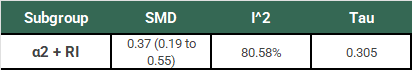
Ok, so we have our SMD of 0.37 (95% CI: 0.19 to 0.55). Remember that this study used a random-effects model, so this is an estimate of the mean of the distribution of “true” effects of the 18 studies in this subgroup. This estimation does not tell us (1) how much “true” effects vary between studies or (2) what range of “true” effects could be expected in an additional new study. We need to do some more work to understand the clinical significance of this result.
Looking at I2 we know that 80.58% of the variation between our study results are due to real differences, but we don’t know how big those differences are yet. Using τ, we calculate a 95% PI of -0.298 to 1.038. In plain English:
If we did one additional study that was similar to the 18 already included in this subgroup, there is a 95% chance that the “true” effect (SMD) of that study would fall between -0.298 to 1.038.
The following table has the results of this same analysis for all of the α2-antagonist subgroups for comparison:
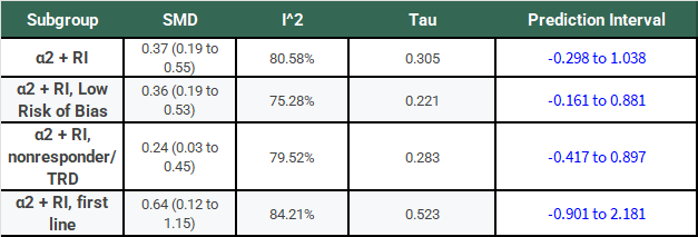
Notice that, for all of these subgroups, the large I2 has not gone away, τ is large relative to the SMD, and the 95% PIs cross 0.
If we’re going to take a frequentist perspective, I would say that it seems like a bit of a problem that all of the PI’s cross 0 and do so rather substantially! Don’t we normally describe 95% confidence intervals that cross 0 as not reaching statistical significance? Why shouldn’t we treat a PI the same way?
The authors try and explain this away — I think quite poorly — in their discussion section by saying things like:
First, I2 values indicated substantial heterogeneity of effects. However, heterogeneity is known to increase with accumulating numbers.
Sure, but that’s why we have τ.
Additional τ statistics were calculated, indicating a spread of data not unfamiliar in medical studies: the standard deviation was lower than or had the same order of magnitude as the effect size.
This is basically saying that we shouldn’t worry about a paper where SMD=1.0 and τ=0.90 because τ is one order of magnitude smaller than the SMD.
You might wonder if I’m being too hard on the authors here. Well, there’s a paper by Rhodes et al. that tells us the τ distribution for mental health outcomes has a median of 0.221 and an IQR of 0.11 to 0.492. So, almost all of the τ values in this study are above the median. More importantly, other studies having similar τ values does not suddenly make the results here less heterogeneous, it just means that there is a lot of heterogeneity in meta-analyses of mental health outcomes.
Nevertheless, as in most meta-analyses, included studies were not homogenous in their design, eg, with differences in blinding status or in the definition of nonresponse to previous antidepressant treatment. As a consequence, we applied random-effects models and showed that results remained robust after each study was left out.
This just means that their SMD didn’t change all that much when they did the leave-one-out analysis! It doesn’t explain the heterogeneity or address the problem of how large τ is! (I’ll get to the random-effects model bit later.)
Further, dichotomizing criteria of treatment success in subgroup analyses, as in remission and response, supported the main results and explained large parts of the between-study heterogeneity.
Yes, dichotomizing criteria supported the main results and reduced I2 by large amounts. (Be careful to note that remission and response are reported as odds-ratios not SMDs!):
The problem is that the starting I2 values were so high that 20-40% reductions still leave you with high I2 values. Also they didn’t report τ, so we have no idea if this reduction in heterogeneity corresponds to a narrowing of the prediction interval, since they are not guaranteed to move in concert.
At this point, I’d be remiss to not include the thoughts of Dr. Kevin Kennedy who offers some very astute criticisms of Henssler:
There are reasons clinicians should be cautious about this result. The authors included 18 studies in their analysis of α2-antagonists, with 10 studies on mirtazapine, six on mianserin, and two on trazodone (which may have only modest α2-antagonism at the doses used in these studies.) The majority of these studies were quite small, but five were robust and included 1,647, 665, 480, 293, and 204 subjects. All five of these large studies were negative. By contrast, the five largest positive studies included only 105, 103, 61, 60, and 47 subjects, with 77, 32, 21, 30, and 21 subjects in the combination medication arms, respectively.
When numerous large, well-designed designed trials consistently find no benefit to α2-antagonist combination therapy, we should be cautious to accept positive results from a meta-analysis whose effect appears to be driven by far smaller studies, especially when the results are highly heterogeneous (I2 = 80.6%) and reflect significant small-study effects and publication bias. The authors’ effort to correct for publication bias resulted in a very modest effect size of 0.19 with marginal statistical significance (95% CI, 0.01–0.36).
When I was first doing the reading for this essay and still hadn’t quite gotten my mind around fixed vs. random-effects modeling, this critique made sense in an intuitive sort of way, but I still felt uneasy. Isn’t the whole point of a meta-analysis to pool all of this data together and treat it like one big study so we don’t have to worry too much about study sizes and the like?
Now that I (and you!) have a better understanding of τ and random-effects models, his concerns are far more legible in concrete, statistical terms. We should now understand that random-effects models will heavily downplay the effects of large, precise studies and amplify the effects of small, imprecise studies with large effect sizes.
As Dr. Kennedy points out, the 5 largest studies of RI+α2 treatment were all negative from a clinical point of view. Kessler et al. had a statistically significant, but clinically negligible positive result of SMD = 0.102 (95% CI: 0.018 to 0.186) in favor of combination therapy.
The studies with the largest effect sizes tend to be the smallest. Of the 7 studies with the largest positive effect sizes, no individual study had more than 61 participants in all treatment arms combined! Some of them also seem unlikely to be relevant to the question being asked. The monotherapy arm for Maes et al. (1996), which was the smallest (n = 21) and had the largest effect size (SMD = 1.548) was only 100mg of trazodone! 100mg! That’s probably not even an antidepressant dose for most people! Why was this study even included?
Given that this is a random-effects analysis, we should also recall that the SMD for this paper tells us about the average “true” effect size for the papers included in the analysis. Why am I reminding you about this?
Assume that the finding in Maes (1996) was accurate; adding fluoxetine 20mg qDay to 100mg of trazodone really does produce an average effect-size of 1.548 in individuals that match the original 22 patients exactly. Assume, also, that the findings in Kato et al. are exactly right, and combination therapy of sertraline + mirtazapine really does produce an average effect size of 0.102 in individuals that match the 1647 patients exactly.
How clinically useful is it for you to know where the weighted average of the “true” effect size between those two papers is, when you know that the Kato study is only weighted 3x more than the Maes study? If I added 10 more studies like Maes to the pool, would that average be any more clinically useful? I’d argue that I wouldn’t really want the Maes study included at all!
But I’m being somewhat unfair. This is an extreme example to get you thinking, so let’s be a little more reasonable.
Remember, we’ve calculated the PI for each of these subgroups. Also remember that the PI tells us about what the range of “true” effect sizes we could expect to see if we did an additional study similar to the other studies.
Let’s say that our threshold for being “clearly superior” in a clinical sense is a difference of at least SMD = 0.2 between monotherapy and combination therapy groups. Applying that threshold to the PIs, we can make the following table:
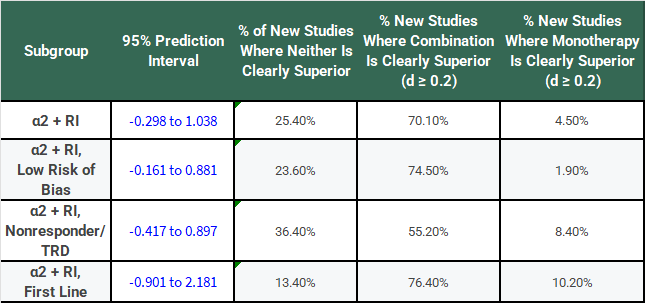
This looks a bit better for combination treatment with α2-antagonists, doesn’t it? You might be willing to roll the dice pretty frequently with a 70% chance of getting a result where SMD >= 0.2 if there’s only a 4.5% chance that monotherapy is meaningfully superior.
But… what would a study with a SMD >= 0.2 look like? From a frequentist perspective, we would look at our 95% PI and say only that such a study would be “interchangeable” with the current studies in our subgroup. That is, we should assume that effect heterogeneity is unrelated to study size or precision.
From a Bayesian perspective, however, we know this to be empirically false. Although the random-effects PI includes large effect sizes, those effects are driven almost entirely by small, imprecise studies. Empirically, large effects have only been observed in those sorts of studies, so a future study showing a large effect would most plausibly share similar design characteristics (e.g. small sample size).
We also have to grapple with whether or not we think the weights assigned through the random-effects model are reasonable given what we know about the studies themselves. In other words, it is reasonable that e.g. the Kato et al. study, is weighted only 3x more than Maes (1996)? That seems like a pretty difficult argument to make.
Finally, there is also the issue of publication bias that Dr. Kennedy brings up in the critique I quoted above. Here is the result pulled from the paper itself:
For RI+α2 analyses, an Egger test result was positive (P = .02, df = 16). A trim-and-fill procedure (Duval and Tweedie) with 6 studies trimmed to the left of the mean resulted in a reduced effect size that was still statistically significant (0.19; 95% CI, 0.01-0.36).
Unfortunately, the authors did not include the funnel plot for the RI+α2 analyses in their supplement, so we can’t see which 6 studies were trimmed, but it seems pretty reasonable to assume that they were the ones with the highest variance.
The fact that the SMD comes down to 0.19 (previously the bottom of the original 95% CI!) and is just barely above 0.0 I think gives a good indication of just how strongly these results were driven by small, high variance studies.
But Should We Supplement With Alpha2-Antagonists?
Before you read this meta-analysis, you probably should’ve read the literature, seen that the largest trials were negative or very weakly positive, seen that the strongest positive trials were small and imprecise, and come to a conclusion something like this:
For most patients, augmentation is unlikely to provide clinically relevant improvement as long as they’re on a reasonable dose of a SRI/SNRI. The small studies have a lot of variance, but they’re generally of good quality and indicate that there are probably a subset of patients who will experience a clinically meaningful improvement… we just don’t really know who those people are.
After this paper, I think we mostly end up in the same spot.
It still seems likely that there are a subset of patients who will respond to adjunctive mirtazapine, but this study doesn’t really help us identify who they are. Sure, the CI and PI look better for first-line patients, but they only represent 5 of the 18 studies and it is not a good sign that Rush et al. which accounts for 665 of the 905 patients across all 5 of those studies had a SMD=0.037 (95% CI: -0.149 to 0.223).
I absolutely do not think that this study comes anywhere near justifying starting every patient with MDD on adjunctive mirtazapine on the theory that there is a clear benefit in efficacy. There might be some subpopulations out there that should be, but we have to find and define them first.
Citalopram, escitalopram, fluoxetine, paroxetine, and sertraline
For American readers, this equates to mirtazapine. Otherwise this also encompasses mianserin
No, legal doesn’t know about this. No, we’re not going to tell them.
Wow!
In reality you wouldn’t just combine them, but more on that later.
You can’t tell if she’s joking
Remember that 95% CI’s are just 2σ
Similar hides a lot of statistical nuance, but don’t worry about it too much for now. We’ll talk more about it later.
Standard deviation on the other hand, describes the spread or variability in your actual data. It tells you how much individual observations differ from the mean. If you measure the heights of 100 people, the SD tells you how much height varies person-to-person in your sample. Larger SD means more spread-out data. SD doesn't change much with sample size (it's a property of the population); SE decreases as sample size increases (larger samples give more precise estimates)
Sound familiar?
I really enjoyed the statistics overview in this essay! Fascinating. Thank you
Interesting paper. I have encountered patients in a hospital sending tending to gain weight when mirtazapine is added, perhaps due to a combination of a sedentary lifestyle and mirtazapine’s purported effects on shifting dietary carbohydrate preferences (see Hennings et al., 2019)